One of the most important parts of the Apache Beam ecosystem is its quickly growing set of connectors that allow Beam pipelines to read and write data to various data storage systems (“IOs”). Currently, Beam ships over 20 IO connectors with many more in active development. As user demands for IO connectors grew, our work on improving the related Beam APIs (in particular, the Source API) produced an unexpected result: a generalization of Beam’s most basic primitive, DoFn.

Note to reader

Hello reader! This blog is a great introduction to Splittable DoFns, but was written while the documentation was catching up. After reading this, you can continue your learning on what Splittable DoFns are and how to implement one in the official Beam Documentation.

Connectors as mini-pipelines

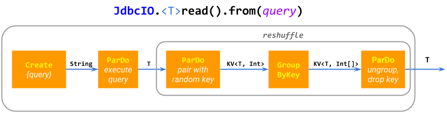
One of the main reasons for this vibrant IO connector ecosystem is that developing a basic IO is relatively straightforward: many connector implementations are simply mini-pipelines (composite PTransforms) made of the basic Beam ParDo and GroupByKey primitives. For example, ElasticsearchIO.write() expands into a single ParDo with some batching for performance; JdbcIO.read() expands into Create.of(query), a reshuffle to prevent fusion, and ParDo(execute sub-query). Some IOs construct considerably more complicated pipelines.

This “mini-pipeline” approach is flexible, modular, and generalizes to data sources that read from a dynamically computed PCollection of locations, such as SpannerIO.readAll() which reads the results of a PCollection of queries from Cloud Spanner, compared to SpannerIO.read() which executes a single query. We believe such dynamic data sources are a very useful capability, often overlooked by other data processing frameworks.

When ParDo and GroupByKey are not enough

Despite the flexibility of ParDo, GroupByKey and their derivatives, in some cases building an efficient IO connector requires extra capabilities.

For example, imagine reading files using the sequence ParDo(filepattern → expand into files), ParDo(filename → read records), or reading a Kafka topic using ParDo(topic → list partitions), ParDo(topic, partition → read records). This approach has two big issues:

• In the file example, some files might be much larger than others, so the second ParDo may have very long individual @ProcessElement calls. As a result, the pipeline can suffer from poor performance due to stragglers.

• In the Kafka example, implementing the second ParDo is simply impossible with a regular DoFn, because it would need to output an infinite number of records per each input element topic, partition (stateful processing comes close, but it has other limitations that make it insufficient for this task).

Beam Source API

Apache Beam historically provides a Source API (BoundedSource and UnboundedSource) which does not have these limitations and allows development of efficient data sources for batch and streaming systems. Pipelines use this API via the Read.from(Source) built-in PTransform.

The Source API is largely similar to that of most other data processing frameworks, and allows the system to read data in parallel using multiple workers, as well as checkpoint and resume reading from an unbounded data source. Additionally, the Beam BoundedSource API provides advanced features such as progress reporting and dynamic rebalancing (which together enable autoscaling), and UnboundedSource supports reporting the source’s watermark and backlog (until SDF, we believed that “batch” and “streaming” data sources are fundamentally different and thus require fundamentally different APIs).

Unfortunately, these features come at a price. Coding against the Source API involves a lot of boilerplate and is error-prone, and it does not compose well with the rest of the Beam model because a Source can appear only at the root of a pipeline. For example:

• Using the Source API, it is not possible to read a PCollection of filepatterns.

• A Source can not read a side input, or wait on another pipeline step to produce the data.

• A Source can not emit an additional output (for example, records that failed to parse) and so on.

The Source API is not composable even with itself. For example, suppose Alice implements an unbounded Source that watches a directory for new matching files, and Bob implements an unbounded Source that tails a file. The Source API does not let them simply chain the sources together and obtain a Source that returns new records in new log files in a directory (a very common user request). Instead, such a source would have to be developed mostly from scratch, and our experience shows that a full-featured monolithic implementation of such a Source is incredibly difficult and error-prone.

Another class of issues with the Source API comes from its strict bounded/unbounded dichotomy:

• It is difficult or impossible to reuse code between seemingly very similar bounded and unbounded sources, for example, the BoundedSource that generates a sequence [a, b) and the UnboundedSource that generates a sequence [a, inf) don’t share any code in the Beam Java SDK.

• It is not clear how to classify the ingestion of a very large and continuously growing dataset. Ingesting its “already available” part seems to require a BoundedSource: the runner could benefit from knowing its size, and could perform dynamic rebalancing. However, ingesting the continuously arriving new data seems to require an UnboundedSource for providing watermarks. From this angle, the Source API has the same issues as Lambda Architecture.

About two years ago we began thinking about how to address the limitations of the Source API, and ended up, surprisingly, addressing the limitations of DoFn instead.

Enter Splittable DoFn

Splittable DoFn (SDF) is a generalization of DoFn that gives it the core capabilities of Source while retaining DoFn’s syntax, flexibility, modularity, and ease of coding. As a result, it becomes possible to develop more powerful IO connectors than before, with shorter, simpler, more reusable code.

Note that, unlike Source, SDF does not have distinct bounded/unbounded APIs, just as regular DoFns don’t: there is only one API, which covers both of these use cases and anything in between. Thus, SDF closes the final gap in the unified batch/streaming programming model of Apache Beam.

When reading the explanation of SDF below, keep in mind the running example of a DoFn that takes a filename as input and outputs the records in that file. People familiar with the Source API may find it useful to think of SDF as a way to read a PCollection of sources, treating the source itself as just another piece of data in the pipeline (this, in fact, was one of the early design iterations among the work that led to creation of SDF).

The two aspects where Source has an advantage over a regular DoFn are:

• Splittability: applying a DoFn to a single element is monolithic, but reading from a Source is non-monolithic. The whole Source doesn’t have to be read at once; rather, it is read in parts, called bundles. For example, a large file is usually read in several bundles, each reading some sub-range of offsets within the file. Likewise, a Kafka topic (which, of course, can never be read “fully”) is read over an infinite number of bundles, each reading some finite number of elements.

• Interaction with the runner: runners apply a DoFn to a single element as a “black box”, but interact quite richly with Source. Source provides the runner with information such as its estimated size (or its generalization, “backlog”), progress through reading the bundle, watermarks etc. The runner uses this information to tune the execution and control the breakdown of the Source into bundles. For example, a slowly progressing large bundle of a file may be dynamically split by a batch-focused runner before it becomes a straggler, and a latency-focused streaming runner may control how many elements it reads from a source in each bundle to optimize for latency vs. per-bundle overhead.

Non-monolithic element processing with restrictions

Splittable DoFn supports Source-like features by allowing the processing of a single element to be non-monolithic.

The processing of one element by an SDF is decomposed into a (potentially infinite) number of restrictions, each describing some part of the work to be done for the whole element. The input to an SDF’s @ProcessElement call is a pair of an element and a restriction (compared to a regular DoFn, which takes just the element).

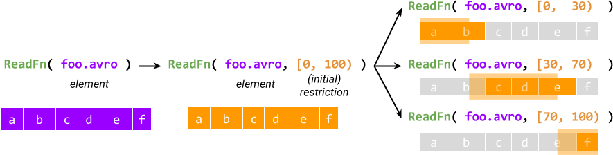
Processing of every element starts by creating an initial restriction that describes the entire work, and the initial restriction is then split further into sub-restrictions which must logically add up to the original. For example, for a splittable DoFn called ReadFn that takes a filename and outputs records in the file, the restriction may be a pair of starting and ending byte offset, and ReadFn may interpret it as read records whose starting offsets are in the given range.

The idea of restrictions provides non-monolithic execution - the first ingredient for parity with Source. The other ingredient is interaction with the runner: the runner has access to the restriction of each active @ProcessElement call of an SDF, can inquire about the progress of the call, and most importantly, can split the restriction while it is being processed (hence the name Splittable DoFn).

Splitting produces a primary and residual restriction that add up to the original restriction being split: the current @ProcessElement call keeps processing the primary, and the residual will be processed by another @ProcessElement call. For example, a runner may schedule the residual to be processed in parallel on another worker.

Splitting of a running @ProcessElement call has two critically important uses:

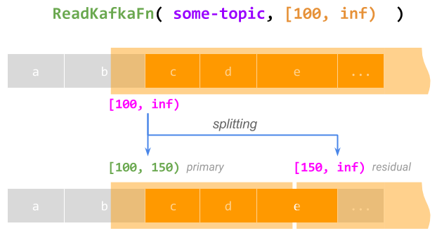
• Supporting infinite work per element. A restriction is, in general, not required to describe a finite amount of work. For example, reading from a Kafka topic starting from offset 100 can be represented by the restriction [100, inf). A @ProcessElement call processing this entire restriction would, of course, never complete. However, while such a call runs, a runner can split the restriction into a finite primary [100, 150) (letting the current call complete this part) and an infinite residual [150, inf) to be processed later, effectively checkpointing and resuming the call; this can be repeated forever.

• Dynamic rebalancing. When a (typically batch-focused) runner detects that a @ProcessElement call is going to take too long and become a straggler, it can split the restriction in some proportion so that the primary is short enough to not be a straggler, and can schedule the residual in parallel on another worker. For details, see No Shard Left Behind.

Logically, the execution of an SDF on an element works according to the following diagram, where “magic” stands for the runner-specific ability to split the restrictions and schedule processing of residuals.

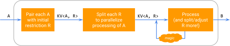
This diagram emphasizes that splittability is an implementation detail of the particular DoFn: a splittable DoFn still looks like a DoFn<A, B> to its user, and can be applied via a ParDo to a PCollection<A> producing a PCollection<B>.

Which DoFns need to be splittable

Note that decomposition of an element into element/restriction pairs is not automatic or “magical”: SDF is a new API for authoring a DoFn, rather than a new way to execute an existing DoFn. When making a DoFn splittable, the author needs to:

• Consider the structure of the work it does for every element.

• Come up with a scheme for describing parts of this work using restrictions.

• Write code for creating the initial restriction, splitting it, and executing an element/restriction pair.

An overwhelming majority of DoFns found in user pipelines do not need to be made splittable: SDF is an advanced, powerful API, primarily targeting authors of new IO connectors (though it has interesting non-IO applications as well: see Non-IO examples).

Execution of a restriction and data consistency

One of the most important parts of the Splittable DoFn design is related to how it achieves data consistency while splitting. For example, while the runner is preparing to split the restriction of an active @ProcessElement call, how can it be sure that the call has not concurrently progressed past the point of splitting?

This is achieved by requiring the processing of a restriction to follow a certain pattern. We think of a restriction as a sequence of blocks - elementary indivisible units of work, identified by a position. A @ProcessElement call processes the blocks one by one, first claiming the block’s position to atomically check if it’s still within the range of the restriction, until the whole restriction is processed.

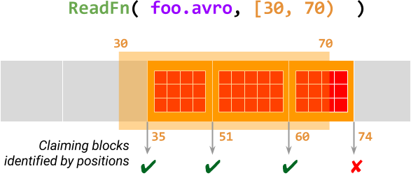
The diagram below illustrates this for ReadFn (a splittable DoFn that reads Avro files) processing the element foo.avro with restriction [30, 70). This @ProcessElement call scans the Avro file for data blocks starting from offset 30 and claims the position of each block in this range. If a block is claimed successfully, then the call outputs all records in this data block, otherwise, it terminates.

For more details, see Restrictions, blocks and positions in the design proposal document.

Code example

Let us look at some examples of SDF code. The examples use the Beam Java SDK, which represents splittable DoFns as part of the flexible annotation-based DoFn machinery, and the proposed SDF syntax for Python.

• A splittable DoFn is a DoFn - no new base class needed. Any SDF derives from the DoFn class and has a @ProcessElement method.

• The @ProcessElement method takes an additional RestrictionTracker parameter that gives access to the current restriction in addition to the current element.

• An SDF needs to define a @GetInitialRestriction method that can create a restriction describing the complete work for a given element.

• There are several less important optional methods, such as @SplitRestriction for pre-splitting the initial restriction into several smaller restrictions, and a few others.

The “Hello World” of SDF is a counter, which takes pairs (x, N) as input and produces pairs (x, 0), (x, 1), …, (x, N-1) as output.

class CountFn<T> extends DoFn<KV<T, Long>, KV<T, Long>> {
  @ProcessElement
  public void process(ProcessContext c, OffsetRangeTracker tracker) {
    for (long i = tracker.currentRestriction().getFrom(); tracker.tryClaim(i); ++i) {
      c.output(KV.of(c.element().getKey(), i));
    }
  }

  @GetInitialRestriction
  public OffsetRange getInitialRange(KV<T, Long> element) {
    return new OffsetRange(0L, element.getValue());
  }
}

PCollection<KV<String, Long>> input = …;
PCollection<KV<String, Long>> output = input.apply(
    ParDo.of(new CountFn<String>());

class CountFn(DoFn):
  def process(element, tracker=DoFn.RestrictionTrackerParam)
    for i in xrange(*tracker.current_restriction()):
      if not tracker.try_claim(i):
        return
      yield element[0], i

  def get_initial_restriction(element):
    return (0, element[1])

This short DoFn subsumes the functionality of CountingSource, but is more flexible: CountingSource generates only one sequence specified at pipeline construction time, while this DoFn can generate a dynamic family of sequences, one per element in the input collection (it does not matter whether the input collection is bounded or unbounded).

However, the Source-specific capabilities of CountingSource are still available in CountFn. For example, if a sequence has a lot of elements, a batch-focused runner can still apply dynamic rebalancing to it and generate different subranges of the sequence in parallel by splitting the OffsetRange. Likewise, a streaming-focused runner can use the same splitting logic to checkpoint and resume the generation of the sequence even if it is, for practical purposes, infinite (for example, when applied to a KV(..., Long.MAX_VALUE)).

A slightly more complex example is the ReadFn considered above, which reads data from Avro files and illustrates the idea of blocks: we provide pseudocode to illustrate the approach.

class ReadFn extends DoFn<String, AvroRecord> {
  @ProcessElement
  void process(ProcessContext c, OffsetRangeTracker tracker) {
    try (AvroReader reader = Avro.open(filename)) {
      // Seek to the first block starting at or after the start offset.
      reader.seek(tracker.currentRestriction().getFrom());
      while (reader.readNextBlock()) {
        // Claim the position of the current Avro block
        if (!tracker.tryClaim(reader.currentBlockOffset())) {
          // Out of range of the current restriction - we're done.
          return;
        }
        // Emit all records in this block
        for (AvroRecord record : reader.currentBlock()) {
          c.output(record);
        }
      }
    }
  }

  @GetInitialRestriction
  OffsetRange getInitialRestriction(String filename) {
    return new OffsetRange(0, new File(filename).getSize());
  }
}

class AvroReader(DoFn):
  def process(filename, tracker=DoFn.RestrictionTrackerParam)
    with fileio.ChannelFactory.open(filename) as file:
      start, stop = tracker.current_restriction()
      # Seek to the first block starting at or after the start offset.
      file.seek(start)
      block = AvroUtils.get_next_block(file)
      while block:
        # Claim the position of the current Avro block
        if not tracker.try_claim(block.start()):
          # Out of range of the current restriction - we're done.
          return
        # Emit all records in this block
        for record in block.records():
          yield record
        block = AvroUtils.get_next_block(file)

  def get_initial_restriction(self, filename):
    return (0, fileio.ChannelFactory.size_in_bytes(filename))

This hypothetical DoFn reads records from a single Avro file. Notably missing is the code for expanding a filepattern: it no longer needs to be part of this DoFn! Instead, the SDK includes a FileIO.matchAll() transform for expanding a filepattern into a PCollection of filenames, and different file format IOs can reuse the same transform, reading the files with different DoFns.

This example demonstrates the benefits of increased modularity allowed by SDF: FileIO.matchAll() supports continuous ingestion of new files in streaming pipelines using .continuously(), and this functionality becomes automatically available to various file format IOs. For example, TextIO.read().watchForNewFiles() uses FileIO.matchAll() under the hood).

Current status

Splittable DoFn is a major new API, and its delivery and widespread adoption involves a lot of work in different parts of the Apache Beam ecosystem. Some of that work is already complete and provides direct benefit to users via new IO connectors. However, a large amount of work is in progress or planned.

As of August 2017, SDF is available for use in the Beam Java Direct runner and Dataflow Streaming runner, and implementation is in progress in the Flink and Apex runners; see capability matrix for the current status. Support for SDF in the Python SDK is in active development.

Several SDF-based transforms and IO connectors are available for Beam users at HEAD and will be included in Beam 2.2.0. TextIO and AvroIO finally provide continuous ingestion of files (one of the most frequently requested features) via .watchForNewFiles() which is backed by the utility transforms FileIO.matchAll().continuously() and the more general Watch.growthOf(). These utility transforms are also independently useful for “power user” use cases.

To enable more flexible use cases for IOs currently based on the Source API, we will change them to use SDF. This transition is pioneered by TextIO and involves temporarily executing SDF via the Source API to support runners lacking the ability to run SDF directly.

In addition to enabling new IOs, work on SDF has influenced our thinking about other parts of the Beam programming model:

• SDF unified the final remaining part of the Beam programming model that was not batch/streaming agnostic (the Source API). This led us to consider use cases that cannot be described as purely batch or streaming (for example, ingesting a large amount of historical data and carrying on with more data arriving in real time) and to develop a unified notion of “progress” and “backlog”.

• The Fn API - the foundation of Beam’s future support for cross-language pipelines - uses SDF as the only concept representing data ingestion.

• Implementation of SDF has lead to formalizing pipeline termination semantics and making it consistent between runners.

• SDF set a new standard for how modular IO connectors can be, inspiring creation of similar APIs for some non-SDF-based connectors (for example, SpannerIO.readAll() and the planned JdbcIO.readAll()).

Call to action

Apache Beam thrives on having a large community of contributors. Here are some ways you can get involved in the SDF effort and help make the Beam IO connector ecosystem more modular:

• Use the currently available SDF-based IO connectors, provide feedback, file bugs, and suggest or implement improvements.

• Propose or develop a new IO connector based on SDF.

• Implement or improve support for SDF in your favorite runner.

• Subscribe and contribute to the occasional SDF-related discussions on user@beam.apache.org (mailing list for Beam users) and dev@beam.apache.org (mailing list for Beam developers)!