Introduction to the Design of Our Autoscaler for Apache Beam Jobs

Welcome to the third and final part of our blog series on building a scalable, self-managed streaming infrastructure with Beam and Flink. In our previous post, we delved into the scale of our streaming platforms, highlighting our capacity to manage over 40,000 streaming jobs and process upwards of 10 million events per second. This impressive scale sets the stage for the challenge we address today: the intricate task of resource allocation in a dynamic streaming environment.

In this blog post Talat Uyarer (Architect / Senior Principal Engineer) and Rishabh Kedia (Principal Engineer) describe more details about our Autoscaler. Imagine a scenario where your streaming system is inundated with fluctuating workloads. Our case presents a unique challenge, as our customers, equipped with firewalls distributed globally, generate logs at various times of the day. This results in workloads that not only vary by time but also escalate over time due to changes in settings or the addition of new cybersecurity solutions from PANW. Furthermore, updates to our codebase necessitate rolling out changes across all streaming jobs, leading to a temporary surge in demand as the system processes unprocessed data.

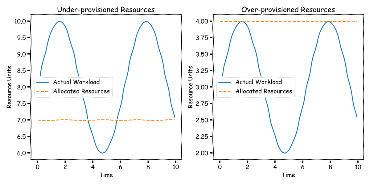
Traditionally, managing this ebb and flow of demand involves a manual, often inefficient approach. One might over-provision resources to handle peak loads, inevitably leading to resource wastage during off-peak hours. Conversely, a more cost-conscious strategy might involve accepting delays during peak times, with the expectation of catching up later. However, both methods demand constant monitoring and manual adjustment - a far from ideal situation.

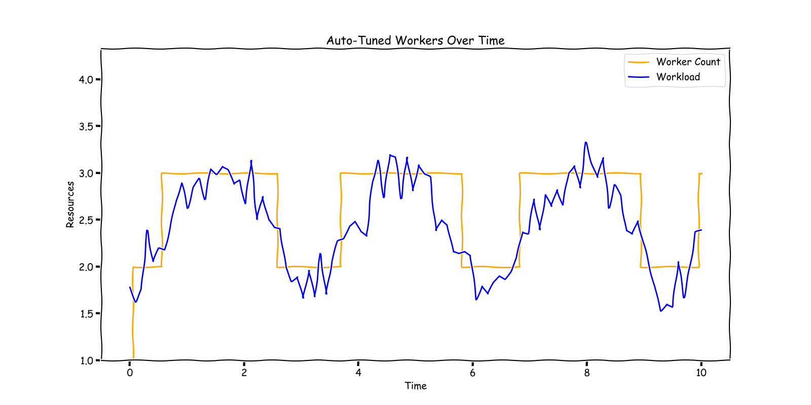
In this modern era, where automated scaling of web front-ends is a given, we aspire to bring the same level of efficiency and automation to streaming infrastructure. Our goal is to develop a system that can dynamically track and adjust to the workload demands of our streaming operations. In this blog post, we will introduce you to our innovative solution - an autoscaler designed specifically for Apache Beam jobs.

For clarity, when we refer to “resources” in this context, we mean the number of Flink Task Managers, or Kubernetes Pods, that process your streaming pipeline. These Task Managers aren’t just about CPU; they also involve RAM, Network, Disk IO, and other computational resources.

However, our solution is predicated on certain assumptions. Primarily, it’s geared towards operations processing substantial data volumes. If your workload only requires a couple of Task Managers, this system might not be the best fit. In Our case we have 10K+ workload and each each of them has different workload. Manual tuning was not an option for us. We also assume that the data is evenly distributed, allowing for increased throughput with the addition of more Task Managers. This assumption is crucial for effective horizontal scaling. While there are real-world complexities that might challenge these assumptions, for the scope of this discussion, we will focus on scenarios where these conditions hold true.

Join us as we delve into the design and functionality of our autoscaler, a solution tailored to bring efficiency, adaptability, and a touch of intelligence to the world of streaming infrastructure.

Identifying the Right Signals for Autoscaling

When we’re overseeing a system like Apache Beam jobs on Flink, it’s crucial to identify key signals that help us understand the relationship between our workload and resources. These signals are our guiding lights, showing us when we’re lagging behind or wasting resources. By accurately identifying these signals, we can formulate effective scaling policies and implement changes in real-time. Imagine needing to expand from 100 to 200 TaskManagers — how do we smoothly make that transition? That’s where these signals come into play.

Remember, we’re aiming for a universal solution applicable to any workload and pipeline. While specific problems might benefit from unique signals, our focus here is on creating a one-size-fits-all approach.

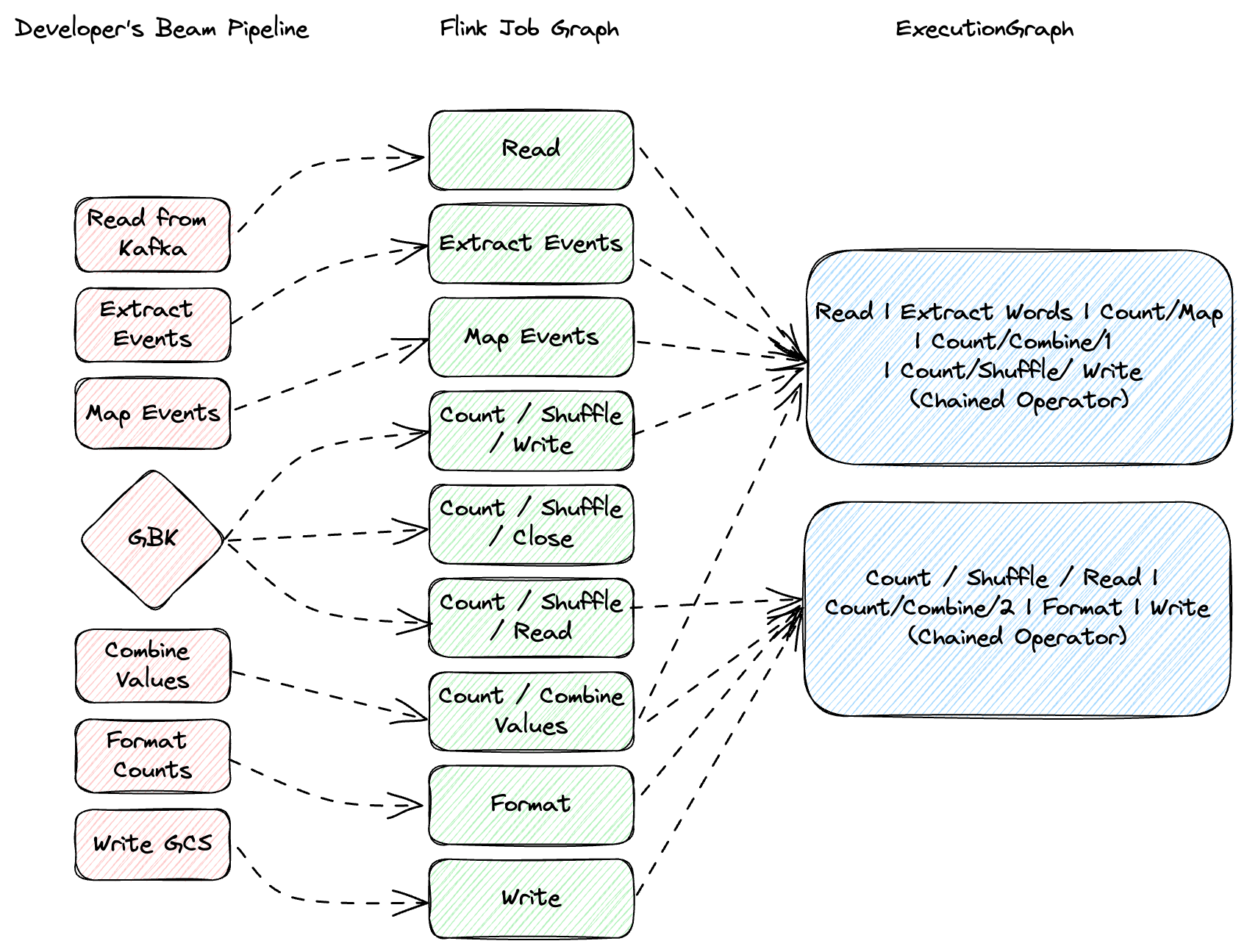
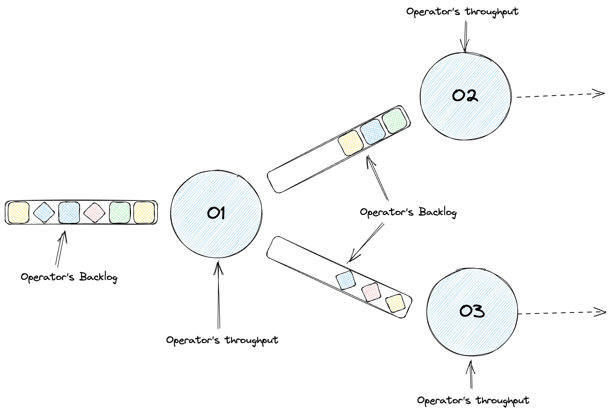
In Flink, tasks form the basic execution unit and consist of one or more operators, such as map, filter, or reduce. Flink optimizes performance by chaining these operators into single tasks when possible, minimizing overheads like thread context switching and network I/O. Your pipeline, when optimized, turns into a directed acyclic graph of stages, each processing elements based on your code. Don’t confuse stages with physical machines — they’re separate concepts. In our job we measure backlog information by using Apache Beam’s backlog_bytes and backlog_elements metrics.

Upscaling Signals

Backlog Growth

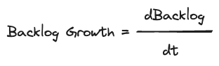
Let’s take a practical example. Consider a pipeline reading from Kafka, where different operators handle data parsing, formatting, and accumulation. The key metric here is throughput — how much data each operstor processes over time. But throughput alone isn’t enough. We need to examine the queue size or backlog at each operator. A growing backlog indicates we’re falling behind. We measure this as backlog growth — the first derivative of backlog size over time, highlighting our processing deficit.

Backlog Time

This leads us to backlog time, a derived metric that compares backlog size with throughput. It’s a measure of how long it would take to clear the current backlog, assuming no new data arrives. This helps us identify if a backlog of a certain size is acceptable or problematic, based on our specific processing needs and thresholds.

Downscaling: When Less is More

CPU Utilization

A key signal for downscaling is CPU utilization. Low CPU utilization suggests we’re using more resources than necessary. By monitoring this, we can scale down efficiently without compromising performance.

Signals Summary

In summary, the signals we’ve identified for effective autoscaling are:

1. Throughput: The baseline of our performance.
2. Backlog Growth: Indicates if we’re keeping pace with incoming data.
3. Backlog Time: Helps understand the severity of backlog.
4. CPU Utilization: Guides us in resource optimization.

These signals might seem straightforward, but their simplicity is key to a scalable, workload-agnostic autoscaling solution.

Simplifying Autoscaling Policies for Apache Beam Jobs on Flink

In the world of Apache Beam jobs running on Flink, deciding when to scale up or down is a bit like being a chef in a busy kitchen. You need to keep an eye on several ingredients — your workload, virtual machines (VMs), and how they interact. It’s about maintaining a perfect balance. Our main goals? Avoid falling behind in processing (no backlog growth), ensure that any existing backlog is manageable (short backlog time), and use our resources (like CPU) efficiently.

Up-scaling: Keeping Up and Catching Up

Imagine your system is like a team of chefs working together. Here’s how we decide when to bring more chefs into the kitchen (a.k.a. upscaling):

1. Keeping Up: First, we look at our current team size (number of VMs) and how much they’re processing (throughput). We then adjust our team size based on the amount of incoming orders (input rate). It’s about ensuring that our team is big enough to handle the current demand.

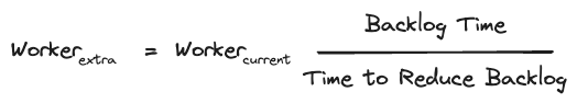
2. Catching Up: Sometimes, we might have a backlog of orders. In that case, we decide how many extra chefs we need to clear this backlog within a desired time (like 60 seconds). This part of the policy helps us get back on track swiftly.

Scaling Example: A Practical Look

Let’s paint a picture with an example. Initially, we have a steady flow of orders (input rate) matching our processing capacity (throughput), so there’s no backlog. But suddenly, orders increase, and our team starts falling behind, creating a backlog. We respond by increasing our team size to match the new rate of orders. Though the backlog doesn’t grow further, it still exists. Finally, we add a few more chefs to the team, which allows us to clear the backlog quickly and return to a new, balanced state.

Downscaling: When to Reduce Resources

Downscaling is like knowing when some chefs can take a break after a rush hour. We consider this when:

• Our backlog is low — we’ve caught up with the orders.
• The backlog isn’t growing — we’re keeping up with incoming orders.
• Our kitchen (CPU) isn’t working too hard — we’re using our resources efficiently.

Downscaling is all about reducing resources without affecting the quality of service. It’s about ensuring that we’re not overstaffed when the rush hour is over.

Summary: A Recipe for Effective Scaling

In summary, our scaling policy is for scale up, we first ensure that the time to drain the backlog is beyond the threshold (120s) or the cpu is above the threshold (90%)

Increasing Backlog aka Backlog Growth > 0 :

Consistent Backlog aka Backlog Growth = 0:

To Sum up:

To scale down, we need to ensure the machine utilization is low (< 70%) and there is no backlog growth and current time to drain backlog is less than the limit (10s)

So the only driving factor to calculate the required resources after a scale down is CPU

Executing Autoscaling Decision

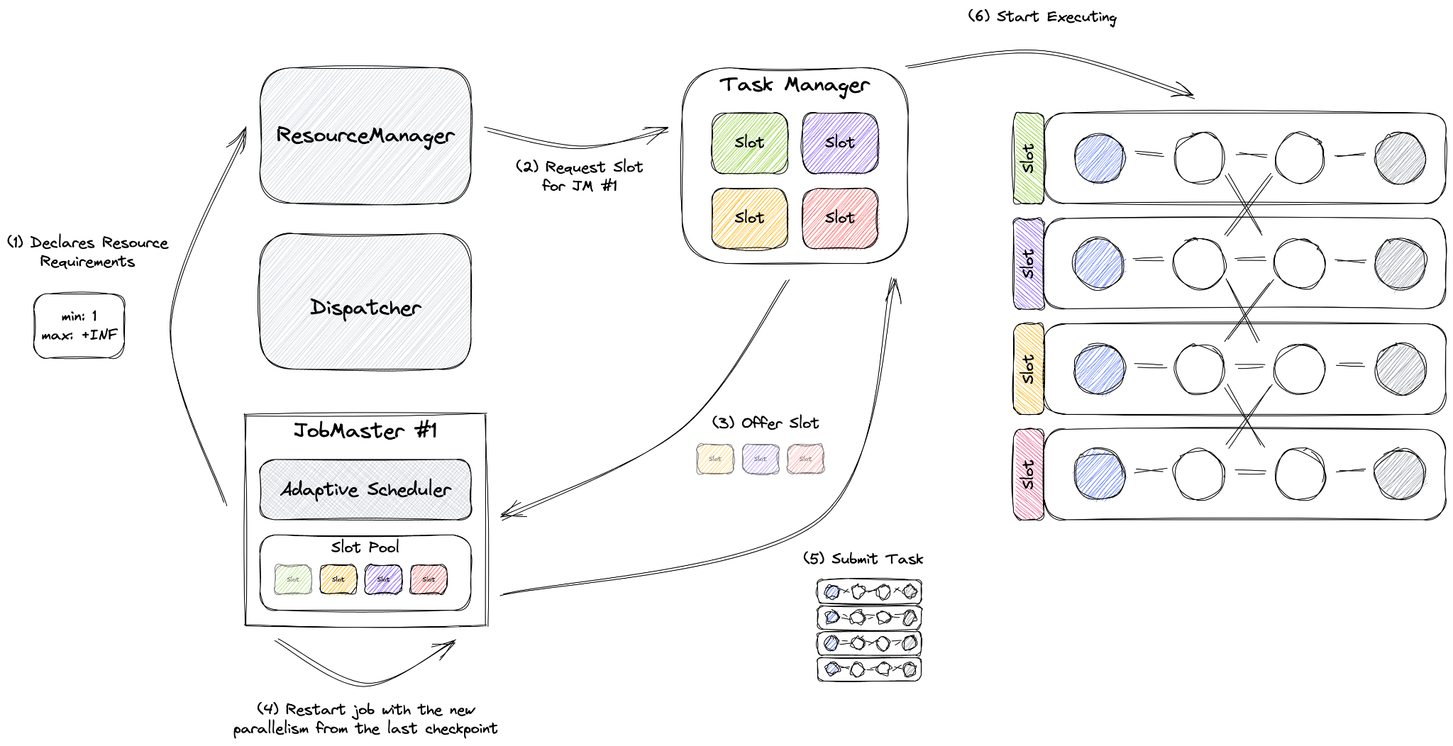
In our setup we use Reactive Mode which uses Adaptive Scheduler and Declarative Resources manager. We wanted to align resources with slots. As advised in most of the Flink documentation we set one per vCPU slot. Most of our jobs use 1 vCPU 4GB Memory combination for TaskManager.

Reactive Mode, a unique feature of the Adaptive Scheduler, operates under the principle of one job per cluster, a rule enforced in Application Mode. In this mode, a job is configured to utilize all available resources within the cluster. Adding a TaskManager will increase the job’s scale, while removing resources will decrease it. In this setup, Flink autonomously manages the job’s parallelism, always maximizing it.

During a rescaling event, Reactive Mode restarts the job using the most recent checkpoint. This eliminates the need for creating a savepoint, typically required for manual job rescaling. The volume of data reprocessed after rescaling is influenced by the checkpointing interval(10 seconds for us), and the time it takes to restore depends on the size of the state.

The scheduler determines the parallelism of each operator within a job. This setting is not user-configurable and any attempts to set it, whether for individual operators or the entire job, will be overlooked.

Parallelism can only be influenced by setting a maximum for pipelines, which the scheduler will honor. Our maxParallelism is limited by the total count of partitions that the pipeline will process, as well as by the job itself. We cap the maximum number of TaskManagers with maxWorker count and control the job’s key count in shuffle by setting maxParallelism. Additionally, we set maxParallelism per pipeline to manage pipeline parallelism. The job cannot exceed the job’s maxParallelism in terms of workers.

After autoscaler analysis, we will tag if the job needs to be scaled up, no action or scaled down. To interact with the job, we use a library we have built over Flink Kubernetes Operator. This library allows us to interact with our flink jobs via a simple java method call. Library will convert our method call to a kubernetes command.

In the kubernetes world, the call will look like this for a scale up:

kubectl scale flinkdeployment job-name --replicas=100

Apache Flink will handle the rest of the work needed to scale up.

Maintaining State for Stateful Streaming Application with Autoscaling

Adapting Apache Flink’s state recovery mechanisms for autoscaling involves leveraging its robust features like max parallelism, checkpointing, and the Adaptive Scheduler to ensure efficient and resilient stream processing, even as the system dynamically adjusts to varying loads. Here’s how these components work together in an autoscaling context:

1. Max Parallelism sets an upper limit on how much a job can scale out, ensuring that state can be redistributed across a larger or smaller number of nodes without exceeding predefined boundaries. This is crucial for autoscaling because it allows Flink to manage state effectively, even as the number of task slots changes to accommodate varying workloads.
2. Checkpointing is at the heart of Flink’s fault tolerance mechanism, periodically saving the state of each job to a durable storage (in our case it is GCS bucket). In an autoscaling scenario, checkpointing enables Flink to recover to a consistent state after scaling operations. When the system scales out (adds more resources) or scales in (removes resources), Flink can restore the state from these checkpoints, ensuring data integrity and processing continuity without losing critical information. In scale down or up situations there could be a moment to reprocess data from last checkpoint. To reduce that amount we reduce the checkpointing interval to 10 seconds.
3. Reactive Mode is a special mode for Adaptive Scheduler, that assumes a single job per-cluster (enforced by the Application Mode). Reactive Mode configures a job so that it always uses all resources available in the cluster. Adding a TaskManager will scale up your job, removing resources will scale it down. Flink will manage the parallelism of the job, always setting it to the highest possible values. When a job undergoes resizing, Reactive Mode triggers a restart using the most recent successful checkpoint.

Conclusion

In this blog series, we’ve taken a deep dive into the creation of an autoscaler for Apache Beam in a high-volume streaming environment, highlighting the journey from conceptualization to implementation. This endeavor not only tackled the complexities of dynamic resource allocation but also set a new standard for efficiency and adaptability in streaming infrastructure. By marrying intelligent scaling policies with the robust capabilities of Apache Beam and Flink, we’ve showcased a scalable solution that optimizes resource use and maintains performance under varying loads. This project stands as a testament to the power of teamwork, innovation, and a forward-thinking approach to streaming data processing. As we wrap up this series, we express our gratitude to all contributors and look forward to the continuous evolution of this technology, inviting the community to join us in further discussions and developments.

References

[1] Streaming Auto-scaling in Google Cloud Dataflow https://www.infoq.com/presentations/google-cloud-dataflow/

[2] Pipeline lifecycle https://cloud.google.com/dataflow/docs/pipeline-lifecycle

[3] Flink Elastic Scaling https://nightlies.apache.org/flink/flink-docs-master/docs/deployment/elastic_scaling/

Acknowledgements

This is a large effort to build the new infrastructure and to migrate the large customer based applications from cloud provider managed streaming infrastructure to self-managed Flink based infrastructure at scale. Thanks the Palo Alto Networks CDL streaming team who helped to make this happen: Kishore Pola, Andrew Park, Hemant Kumar, Manan Mangal, Helen Jiang, Mandy Wang, Praveen Kumar Pasupuleti, JM Teo, Rishabh Kedia, Talat Uyarer, Naitik Dani, and David He.

Explore More:

• Part 1: Introduction to Building and Managing Apache Beam Flink Services on Kubernetes
• Part 2: Build a scalable, self-managed streaming infrastructure with Flink: Tackling Autoscaling Challenges - Part 2

Join the conversation and share your experiences on our Community or contribute to our ongoing projects on GitHub. Your feedback is invaluable. If you have any comments or questions about this series, please feel free to reach out to us via User Mailist

Stay connected with us for more updates and insights into Apache Beam, Flink, and Kubernetes.