


Basics of the Beam model
Apache Beam is a unified model for defining both batch and streaming data-parallel processing pipelines. To get started with Beam, you’ll need to understand an important set of core concepts:
- Pipeline - A pipeline is a user-constructed graph of transformations that defines the desired data processing operations.
- PCollection - A
PCollectionis a data set or data stream. The data that a pipeline processes is part of a PCollection. - PTransform - A
PTransform(or transform) represents a data processing operation, or a step, in your pipeline. A transform is applied to zero or morePCollectionobjects, and produces zero or morePCollectionobjects. - Aggregation - Aggregation is computing a value from multiple (1 or more) input elements.
- User-defined function (UDF) - Some Beam operations allow you to run user-defined code as a way to configure the transform.
- Schema - A schema is a language-independent type definition for
a
PCollection. The schema for aPCollectiondefines elements of thatPCollectionas an ordered list of named fields. - SDK - A language-specific library that lets pipeline authors build transforms, construct their pipelines, and submit them to a runner.
- Runner - A runner runs a Beam pipeline using the capabilities of your chosen data processing engine.
- Window - A
PCollectioncan be subdivided into windows based on the timestamps of the individual elements. Windows enable grouping operations over collections that grow over time by dividing the collection into windows of finite collections. - Watermark - A watermark is a guess as to when all data in a certain window is expected to have arrived. This is needed because data isn’t always guaranteed to arrive in a pipeline in time order, or to always arrive at predictable intervals.
- Trigger - A trigger determines when to aggregate the results of each window.
- State and timers - Per-key state and timer callbacks are lower level primitives that give you full control over aggregating input collections that grow over time.
- Splittable DoFn - Splittable DoFns let you process elements in a non-monolithic way. You can checkpoint the processing of an element, and the runner can split the remaining work to yield additional parallelism.
The following sections cover these concepts in more detail and provide links to additional documentation.
Pipeline
A Beam pipeline is a graph (specifically, a directed acyclic graph) of all the data and computations in your data processing task. This includes reading input data, transforming that data, and writing output data. A pipeline is constructed by a user in their SDK of choice. Then, the pipeline makes its way to the runner either through the SDK directly or through the Runner API’s RPC interface. For example, this diagram shows a branching pipeline:

In this diagram, the boxes represent the parallel computations called PTransforms and the arrows with the circles represent the data (in the form of PCollections) that flows between the transforms. The data might be bounded, stored, data sets, or the data might also be unbounded streams of data. In Beam, most transforms apply equally to bounded and unbounded data.
You can express almost any computation that you can think of as a graph as a
Beam pipeline. A Beam driver program typically starts by creating a Pipeline
object, and then uses that object as the basis for creating the pipeline’s data
sets and its transforms.
For more information about pipelines, see the following pages:
- Beam Programming Guide: Overview
- Beam Programming Guide: Creating a pipeline
- Design your pipeline
- Create your pipeline
PCollection
A PCollection is an unordered bag of elements. Each PCollection is a
potentially distributed, homogeneous data set or data stream, and is owned by
the specific Pipeline object for which it is created. Multiple pipelines
cannot share a PCollection. Beam pipelines process PCollections, and the
runner is responsible for storing these elements.
A PCollection generally contains “big data” (too much data to fit in memory on
a single machine). Sometimes a small sample of data or an intermediate result
might fit into memory on a single machine, but Beam’s computational patterns and
transforms are focused on situations where distributed data-parallel computation
is required. Therefore, the elements of a PCollection cannot be processed
individually, and are instead processed uniformly in parallel.
The following characteristics of a PCollection are important to know.
Bounded vs. unbounded:
A PCollection can be either bounded or unbounded.
- A bounded
PCollectionis a dataset of a known, fixed size (alternatively, a dataset that is not growing over time). Bounded data can be processed by batch pipelines. - An unbounded
PCollectionis a dataset that grows over time, and the elements are processed as they arrive. Unbounded data must be processed by streaming pipelines.
These two categories derive from the intuitions of batch and stream processing, but the two are unified in Beam and bounded and unbounded PCollections can coexist in the same pipeline. If your runner can only support bounded PCollections, you must reject pipelines that contain unbounded PCollections. If your runner is only targeting streams, there are adapters in Beam’s support code to convert everything to APIs that target unbounded data.
Timestamps:
Every element in a PCollection has a timestamp associated with it.
When you execute a primitive connector to a storage system, that connector is responsible for providing initial timestamps. The runner must propagate and aggregate timestamps. If the timestamp is not important, such as with certain batch processing jobs where elements do not denote events, the timestamp will be the minimum representable timestamp, often referred to colloquially as “negative infinity”.
Watermarks:
Every PCollection must have a watermark that estimates how
complete the PCollection is.
The watermark is a guess that “we’ll never see an element with an earlier timestamp”. Data sources are responsible for producing a watermark. The runner must implement watermark propagation as PCollections are processed, merged, and partitioned.
The contents of a PCollection are complete when a watermark advances to
“infinity”. In this manner, you can discover that an unbounded PCollection is
finite.
Windowed elements:
Every element in a PCollection resides in a window. No element
resides in multiple windows; two elements can be equal except for their window,
but they are not the same.
When elements are written to the outside world, they are effectively placed back into the global window. Transforms that write data and don’t take this perspective risk data loss.
A window has a maximum timestamp. When the watermark exceeds the maximum timestamp plus the user-specified allowed lateness, the window is expired. All data related to an expired window might be discarded at any time.
Coder:
Every PCollection has a coder, which is a specification of the binary format
of the elements.
In Beam, the user’s pipeline can be written in a language other than the
language of the runner. There is no expectation that the runner can actually
deserialize user data. The Beam model operates principally on encoded data,
“just bytes”. Each PCollection has a declared encoding for its elements,
called a coder. A coder has a URN that identifies the encoding, and might have
additional sub-coders. For example, a coder for lists might contain a coder for
the elements of the list. Language-specific serialization techniques are
frequently used, but there are a few common key formats (such as key-value pairs
and timestamps) so the runner can understand them.
Windowing strategy:
Every PCollection has a windowing strategy, which is a specification of
essential information for grouping and triggering operations. The Window
transform sets up the windowing strategy, and the GroupByKey transform has
behavior that is governed by the windowing strategy.
For more information about PCollections, see the following page:
PTransform
A PTransform (or transform) represents a data processing operation, or a step,
in your pipeline. A transform is usually applied to one or more input
PCollection objects. Transforms that read input are an exception; these
transforms might not have an input PCollection.
You provide transform processing logic in the form of a function object
(colloquially referred to as “user code”), and your user code is applied to each
element of the input PCollection (or more than one PCollection). Depending on
the pipeline runner and backend that you choose, many different workers across a
cluster might execute instances of your user code in parallel. The user code
that runs on each worker generates the output elements that are added to zero or
more output PCollection objects.
The Beam SDKs contain a number of different transforms that you can apply to
your pipeline’s PCollections. These include general-purpose core transforms,
such as ParDo or Combine. There are also pre-written composite transforms
included in the SDKs, which combine one or more of the core transforms in a
useful processing pattern, such as counting or combining elements in a
collection. You can also define your own more complex composite transforms to
fit your pipeline’s exact use case.
The following list has some common transform types:
- Source transforms such as
TextIO.ReadandCreate. A source transform conceptually has no input. - Processing and conversion operations such as
ParDo,GroupByKey,CoGroupByKey,Combine, andCount. - Outputting transforms such as
TextIO.Write. - User-defined, application-specific composite transforms.
For more information about transforms, see the following pages:
- Beam Programming Guide: Overview
- Beam Programming Guide: Transforms
- Beam transform catalog (Java, Python)
Aggregation
Aggregation is computing a value from multiple (1 or more) input elements. In Beam, the primary computational pattern for aggregation is to group all elements with a common key and window then combine each group of elements using an associative and commutative operation. This is similar to the “Reduce” operation in the MapReduce model, though it is enhanced to work with unbounded input streams as well as bounded data sets.
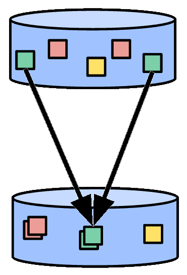
Figure 1: Aggregation of elements. Elements with the same color represent those with a common key and window.
Some simple aggregation transforms include Count (computes the count of all
elements in the aggregation), Max (computes the maximum element in the
aggregation), and Sum (computes the sum of all elements in the aggregation).
When elements are grouped and emitted as a bag, the aggregation is known as
GroupByKey (the associative/commutative operation is bag union). In this case,
the output is no smaller than the input. Often, you will apply an operation such
as summation, called a CombineFn, in which the output is significantly smaller
than the input. In this case the aggregation is called CombinePerKey.
In a real application, you might have millions of keys and/or windows; that is why this is still an “embarrassingly parallel” computational pattern. In those cases where you have fewer keys, you can add parallelism by adding a supplementary key, splitting each of your problem’s natural keys into many sub-keys. After these sub-keys are aggregated, the results can be further combined into a result for the original natural key for your problem. The associativity of your aggregation function ensures that this yields the same answer, but with more parallelism.
When your input is unbounded, the computational pattern of grouping elements by key and window is roughly the same, but governing when and how to emit the results of aggregation involves three concepts:
- Windowing, which partitions your input into bounded subsets that can be complete.
- Watermarks, which estimate the completeness of your input.
- Triggers, which govern when and how to emit aggregated results.
For more information about available aggregation transforms, see the following pages:
- Beam Programming Guide: Core Beam transforms
- Beam Transform catalog (Java, Python)
User-defined function (UDF)
Some Beam operations allow you to run user-defined code as a way to configure
the transform. For example, when using ParDo, user-defined code specifies what
operation to apply to every element. For Combine, it specifies how values
should be combined. By using cross-language transforms,
a Beam pipeline can contain UDFs written in a different language, or even
multiple languages in the same pipeline.
Beam has several varieties of UDFs:
- DoFn - per-element processing
function (used in
ParDo) - WindowFn -
places elements in windows and merges windows (used in
WindowandGroupByKey) - ViewFn - adapts a
materialized
PCollectionto a particular interface (used in side inputs) - WindowMappingFn - maps one element’s window to another, and specifies bounds on how far in the past the result window will be (used in side inputs)
- CombineFn - associative and
commutative aggregation (used in
Combineand state) - Coder - encodes user data; some coders have standard formats and are not really UDFs
Each language SDK has its own idiomatic way of expressing the user-defined functions in Beam, but there are common requirements. When you build user code for a Beam transform, you should keep in mind the distributed nature of execution. For example, there might be many copies of your function running on a lot of different machines in parallel, and those copies function independently, without communicating or sharing state with any of the other copies. Each copy of your user code function might be retried or run multiple times, depending on the pipeline runner and the processing backend that you choose for your pipeline. Beam also supports stateful processing through the stateful processing API.
For more information about user-defined functions, see the following pages:
- Requirements for writing user code for Beam transforms
- Beam Programming Guide: ParDo
- Beam Programming Guide: WindowFn
- Beam Programming Guide: CombineFn
- Beam Programming Guide: Coder
- Beam Programming Guide: Side inputs
Schema
A schema is a language-independent type definition for a PCollection. The
schema for a PCollection defines elements of that PCollection as an ordered
list of named fields. Each field has a name, a type, and possibly a set of user
options.
In many cases, the element type in a PCollection has a structure that can be
introspected. Some examples are JSON, Protocol Buffer, Avro, and database row
objects. All of these formats can be converted to Beam Schemas. Even within a
SDK pipeline, Simple Java POJOs (or equivalent structures in other languages)
are often used as intermediate types, and these also have a clear structure that
can be inferred by inspecting the class. By understanding the structure of a
pipeline’s records, we can provide much more concise APIs for data processing.
Beam provides a collection of transforms that operate natively on schemas. For example, Beam SQL is a common transform that operates on schemas. These transforms allow selections and aggregations in terms of named schema fields. Another advantage of schemas is that they allow referencing of element fields by name. Beam provides a selection syntax for referencing fields, including nested and repeated fields.
For more information about schemas, see the following pages:
Runner
A Beam runner runs a Beam pipeline on a specific platform. Most runners are translators or adapters to massively parallel big data processing systems, such as Apache Flink, Apache Spark, Google Cloud Dataflow, and more. For example, the Flink runner translates a Beam pipeline into a Flink job. The Direct Runner runs pipelines locally so you can test, debug, and validate that your pipeline adheres to the Apache Beam model as closely as possible.
For an up-to-date list of Beam runners and which features of the Apache Beam model they support, see the runner capability matrix.
For more information about runners, see the following pages:
Window
Windowing subdivides a PCollection into windows according to the timestamps
of its individual elements. Windows enable grouping operations over unbounded
collections by dividing the collection into windows of finite collections.
A windowing function tells the runner how to assign elements to one or more
initial windows, and how to merge windows of grouped elements. Each element in a
PCollection can only be in one window, so if a windowing function specifies
multiple windows for an element, the element is conceptually duplicated into
each of the windows and each element is identical except for its window.
Transforms that aggregate multiple elements, such as GroupByKey and Combine,
work implicitly on a per-window basis; they process each PCollection as a
succession of multiple, finite windows, though the entire collection itself may
be of unbounded size.
Beam provides several windowing functions:
- Fixed time windows (also known as “tumbling windows”) represent a consistent duration, non-overlapping time interval in the data stream.
- Sliding time windows (also known as “hopping windows”) also represent time intervals in the data stream; however, sliding time windows can overlap.
- Per-session windows define windows that contain elements that are within a certain gap duration of another element.
- Single global window: by default, all data in a
PCollectionis assigned to the single global window, and late data is discarded. - Calendar-based windows (not supported by the Beam SDK for Python)
You can also define your own windowing function if you have more complex requirements.
For example, let’s say we have a PCollection that uses fixed-time windowing,
with windows that are five minutes long. For each window, Beam must collect all
the data with an event time timestamp in the given window range (between 0:00
and 4:59 in the first window, for instance). Data with timestamps outside that
range (data from 5:00 or later) belongs to a different window.
Two concepts are closely related to windowing and covered in the following sections: watermarks and triggers.
For more information about windows, see the following page:
Watermark
In any data processing system, there is a certain amount of lag between the time a data event occurs (the “event time”, determined by the timestamp on the data element itself) and the time the actual data element gets processed at any stage in your pipeline (the “processing time”, determined by the clock on the system processing the element). In addition, data isn’t always guaranteed to arrive in a pipeline in time order, or to always arrive at predictable intervals. For example, you might have intermediate systems that don’t preserve order, or you might have two servers that timestamp data but one has a better network connection.
To address this potential unpredictability, Beam tracks a watermark. A watermark is a guess as to when all data in a certain window is expected to have arrived in the pipeline. You can also think of this as “we’ll never see an element with an earlier timestamp”.
Data sources are responsible for producing a watermark, and every PCollection
must have a watermark that estimates how complete the PCollection is. The
contents of a PCollection are complete when a watermark advances to
“infinity”. In this manner, you might discover that an unbounded PCollection
is finite. After the watermark progresses past the end of a window, any further
element that arrives with a timestamp in that window is considered late data.
Triggers are a related concept that allow you to modify and refine
the windowing strategy for a PCollection. You can use triggers to decide when
each individual window aggregates and reports its results, including how the
window emits late elements.
For more information about watermarks, see the following page:
Trigger
When collecting and grouping data into windows, Beam uses triggers to determine when to emit the aggregated results of each window (referred to as a pane). If you use Beam’s default windowing configuration and default trigger, Beam outputs the aggregated result when it estimates all data has arrived, and discards all subsequent data for that window.
At a high level, triggers provide two additional capabilities compared to outputting at the end of a window:
- Triggers allow Beam to emit early results, before all the data in a given window has arrived. For example, emitting after a certain amount of time elapses, or after a certain number of elements arrives.
- Triggers allow processing of late data by triggering after the event time watermark passes the end of the window.
These capabilities allow you to control the flow of your data and also balance between data completeness, latency, and cost.
Beam provides a number of pre-built triggers that you can set:
- Event time triggers: These triggers operate on the event time, as indicated by the timestamp on each data element. Beam’s default trigger is event time-based.
- Processing time triggers: These triggers operate on the processing time, which is the time when the data element is processed at any given stage in the pipeline.
- Data-driven triggers: These triggers operate by examining the data as it arrives in each window, and firing when that data meets a certain property. Currently, data-driven triggers only support firing after a certain number of data elements.
- Composite triggers: These triggers combine multiple triggers in various ways. For example, you might want one trigger for early data and a different trigger for late data.
For more information about triggers, see the following page:
State and timers
Beam’s windowing and triggers provide an abstraction for grouping and aggregating unbounded input data based on timestamps. However, there are aggregation use cases that might require an even higher degree of control. State and timers are two important concepts that help with these uses cases. Like other aggregations, state and timers are processed per window.
State:
Beam provides the State API for manually managing per-key state, allowing for
fine-grained control over aggregations. The State API lets you augment
element-wise operations (for example, ParDo or Map) with mutable state. Like
other aggregations, state is processed per window.
The State API models state per key. To use the state API, you start out with a
keyed PCollection. A ParDo that processes this PCollection can declare
persistent state variables. When you process each element inside the ParDo,
you can use the state variables to write or update state for the current key or
to read previous state written for that key. State is always fully scoped only
to the current processing key.
Beam provides several types of state, though different runners might support a different subset of these states.
- ValueState: ValueState is a scalar state value. For each key in the
input, a ValueState stores a typed value that can be read and modified inside
the
DoFn. - A common use case for state is to accumulate multiple elements into a group:
- BagState: BagState allows you to accumulate elements in an unordered bag. This lets you add elements to a collection without needing to read any of the previously accumulated elements.
- MapState: MapState allows you to accumulate elements in a map.
- SetState: SetState allows you to accumulate elements in a set.
- OrderedListState: OrderedListState allows you to accumulate elements in a timestamp-sorted list.
- CombiningState: CombiningState allows you to create a state object that is updated using a Beam combiner. Like BagState, you can add elements to an aggregation without needing to read the current value, and the accumulator can be compacted using a combiner.
You can use the State API together with the Timer API to create processing tasks that give you fine-grained control over the workflow.
Timers:
Beam provides a per-key timer callback API that enables delayed processing of data stored using the State API. The Timer API lets you set timers to call back at either an event-time or a processing-time timestamp. For more advanced use cases, your timer callback can set another timer. Like other aggregations, timers are processed per window. You can use the timer API together with the State API to create processing tasks that give you fine-grained control over the workflow.
The following timers are available:
- Event-time timers: Event-time timers fire when the input watermark for
the
DoFnpasses the time at which the timer is set, meaning that the runner believes that there are no more elements to be processed with timestamps before the timer timestamp. This allows for event-time aggregations. - Processing-time timers: Processing-time timers fire when the real wall-clock time passes. This is often used to create larger batches of data before processing. It can also be used to schedule events that should occur at a specific time.
- Dynamic timer tags: Beam also supports dynamically setting a timer tag. This
allows you to set multiple different timers in a
DoFnand dynamically choose timer tags (for example, based on data in the input elements).
For more information about state and timers, see the following pages:
- Beam Programming Guide: State and Timers
- Stateful processing with Apache Beam
- Timely (and Stateful) Processing with Apache Beam
Splittable DoFn
Splittable DoFn (SDF) is a generalization of DoFn that lets you process
elements in a non-monolithic way. Splittable DoFn makes it easier to create
complex, modular I/O connectors in Beam.
A regular ParDo processes an entire element at a time, applying your regular
DoFn and waiting for the call to terminate. When you instead apply a
splittable DoFn to each element, the runner has the option of splitting the
element’s processing into smaller tasks. You can checkpoint the processing of an
element, and you can split the remaining work to yield additional parallelism.
For example, imagine you want to read every line from very large text files.
When you write your splittable DoFn, you can have separate pieces of logic to
read a segment of a file, split a segment of a file into sub-segments, and
report progress through the current segment. The runner can then invoke your
splittable DoFn intelligently to split up each input and read portions
separately, in parallel.
A common computation pattern has the following steps:
- The runner splits an incoming element before starting any processing.
- The runner starts running your processing logic on each sub-element.
- If the runner notices that some sub-elements are taking longer than others, the runner splits those sub-elements further and repeats step 2.
- The sub-element either finishes processing, or the user chooses to checkpoint the sub-element and the runner repeats step 2.
You can also write your splittable DoFn so the runner can split the unbounded
processing. For example, if you write a splittable DoFn to watch a set of
directories and output filenames as they arrive, you can split to subdivide the
work of different directories. This allows the runner to split off a hot
directory and give it additional resources.
For more information about Splittable DoFn, see the following pages:
What’s next
Take a look at our other documentation such as the Beam programming guide, pipeline execution information, and transform reference catalogs.
Last updated on 2026/02/27
Have you found everything you were looking for?
Was it all useful and clear? Is there anything that you would like to change? Let us know!