Scaling a streaming workload is critical for ensuring that a pipeline can process large amounts of data while also minimizing latency and executing efficiently. Without proper scaling, a pipeline may experience performance issues or even fail entirely, delaying the time to insights for the business.

Given the Apache Beam support for the sources and sinks needed by the workload, developing a streaming pipeline can be easy. You can focus on the processing (transformations, enrichments, or aggregations) and on setting the right configurations for each case.

However, you need to identify the key performance bottlenecks and make sure that the pipeline has the resources it needs to handle the load efficiently. This can involve right-sizing the number of workers, understanding the settings needed for the source and sinks of the pipeline, optimizing the processing logic, and even determining the transport formats.

This article illustrates how to manage the problem of scaling and optimizing a streaming workload developed in Apache Beam and run on Google Cloud using Dataflow. The goal is to reach one million events per second, while also minimizing latency and resource use during execution. The workload uses Pub/Sub as the streaming source and BigQuery as the sink. We describe the reasoning behind the configuration settings and code changes we used to help the workload achieve the desired scale and beyond.

The progression described in this article maps to the evolution of a real-life workload, with simplifications. After the initial business requirements for the pipeline were achieved, the focus shifted to optimizing the performance and reducing the resources needed for the pipeline execution.

Execution setup

For this article, we created a test suite that creates the necessary components for the pipelines to execute. You can find the code in this Github repository. You can find the subsequent configuration changes that are introduced on every run in this folder as scripts that you can run to achieve similar results.

All of the execution scripts can also execute a Terraform-based automation to create a Pub/Sub topic and subscription as well as a BigQuery dataset and table to run the workload. Also, it launches two pipelines: one data generation pipeline that pushes events to the Pub/Sub topic, and an ingestion pipeline that demonstrates the potential improvement points.

In all cases, the pipelines start with an empty Pub/Sub topic and subscription and an empty BigQuery table. The plan is to generate one million events per second and, after a few minutes, review how the ingestion pipeline scales with time. The data being autogenerated is based on provided schemas or IDL (or Interface Description Language) given the configuration, and the goal is to have messages ranging between 800 bytes and 2 KB, adding up to approximately 1 GB/s volume throughput. Also, the ingestion pipelines are using the same worker type configuration on all runs (n2d-standard-4 GCE machines) and are capping the maximum workers number to avoid very large fleets.

All of the executions run on Google Cloud using Dataflow, but you can apply all of the configurations and format changes to the suite while executing on other supported Apache Beam runners. Changes and recommendations are not runner specific.

Local environment requirements

Before launching the startup scripts, install the following items in your local environment:

• gcloud, along with the correct permissions
• Terraform
• JDK 17 or later
• Maven 3.6 or later

For more information, see the requirements section in the GitHub repository.

Also, review the service quotas and resources available in your Google Cloud project. Specifically: Pub/Sub regional capacity, BigQuery ingestion quota, and Compute Engine instances available in the selected region for the tests.

Workload description

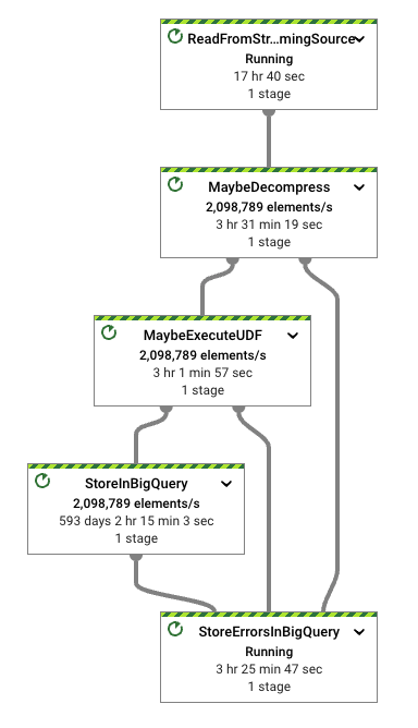
Focusing on the ingestion pipeline, our workload is straightforward. It completes the following steps:

1. reads data in a specific format from Pub/Sub (Apache Thrift in this case)
2. deals with potential compression and batching settings (not enabled by default)
3. executes a UDF (identity function by default)
4. transforms the input format to one of the formats supported by the BigQueryIO transform
5. writes the data to the configured table

The pipeline we used for the tests is highly configurable. For more details about how to tweak the ingestion, see the options in the file. No code changes are needed on any of our steps. The execution scripts take care of the configurations needed.

Although these tests are focused on reading data from Pub/Sub, the ingestion pipeline is capable of reading data from a generic streaming source. The repository contains other examples that show how to launch this same test suite reading data from Pub/Sub Lite and Kafka. In all cases, the pipeline automation sets up the streaming infrastructure.

Finally, you can see in the configuration options that the pipeline supports many transport format options for the input, such as Thrift, Avro, and JSON. This suite focuses on Thrift, because it is a common open source format, and because it generates a format transformation need. The intent is to put some strain in the workload processing. You can run similar tests for Avro and JSON input data. The streaming data generator pipeline can generate random data for the three supported formats by walking directly on the schema (Avro and JSON) or IDL (Thrift) provided for execution.

First run: default settings

The default values for the execution writes the data to BigQuery using STREAMING_INSERTS mode for BigQueryIO. This mode correlates with the tableData insertAll API for BigQuery. This API supports data in JSON format. From the Apache Beam perspective, using the BigQueryIO.writeTableRows method lets us resolve the writes into BigQuery.

For our ingestion pipeline, the Thrift format needs to be transformed into TableRow. To do that, we need to translate the Thrift IDL into a BigQuery table schema. That can be achieved by translating the Thrift IDL into an Avro schema, and then using Beam utilities to translate the table schema for BigQuery. We can do this at bootstrap. The schema transformation is cached at the DoFn level.

After setting up the data generation and ingestion pipelines, and after letting the pipelines run for some minutes, we see that the pipeline is unable to sustain the desired throughput.

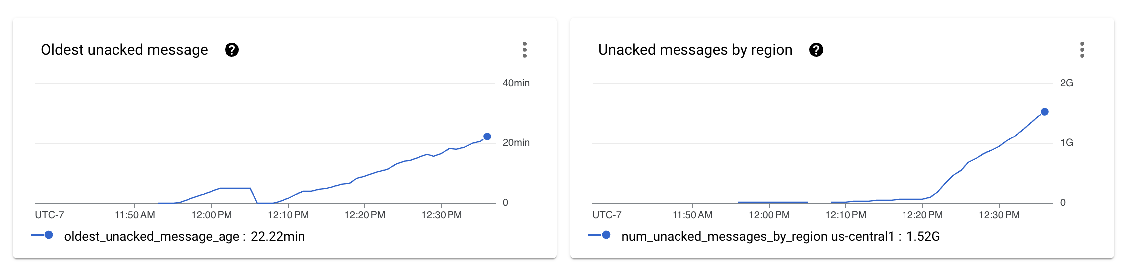
The previous image shows that the number of messages that are not being processed by the ingestion pipeline start to show as unacknowledged messages in Pub/Sub metrics.

Reviewing the per stage performance metrics, we see that the pipeline shows a saw-like shape, which is often associated with the throttling mechanisms the Dataflow runner uses when some of the stages are acting as bottlenecks for the throughput. Also, we see that the Reshuffle step on the BigQueryIO write transform does not scale as expected.

This behavior happens because by default the BigQueryOptions uses 50 different keys to shuffle data to workers before the writes happen on BigQuery. To solve this problem, we can add a configuration to our launch script that enables the write operations to scale to a larger number of workers, which improves performance.

Second run: improve the write bottleneck

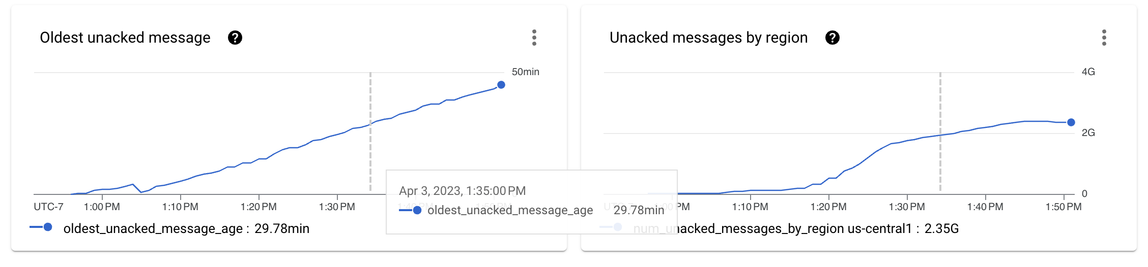
After increasing the number of streaming keys to a higher number, 512 keys in our case, we restarted the test suite. The Pub/Sub metrics started to improve. After an initial ramp on the size of the backlog, the curve started to ease out.

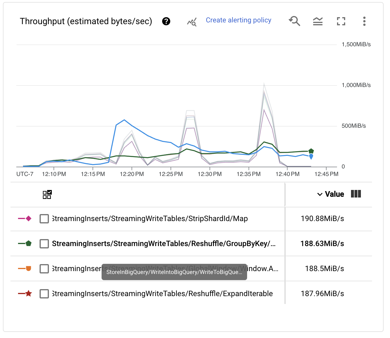
This is good, but we should take a look at the throughput per stage numbers to understand if we are achieving the goal we set up for this exercise.

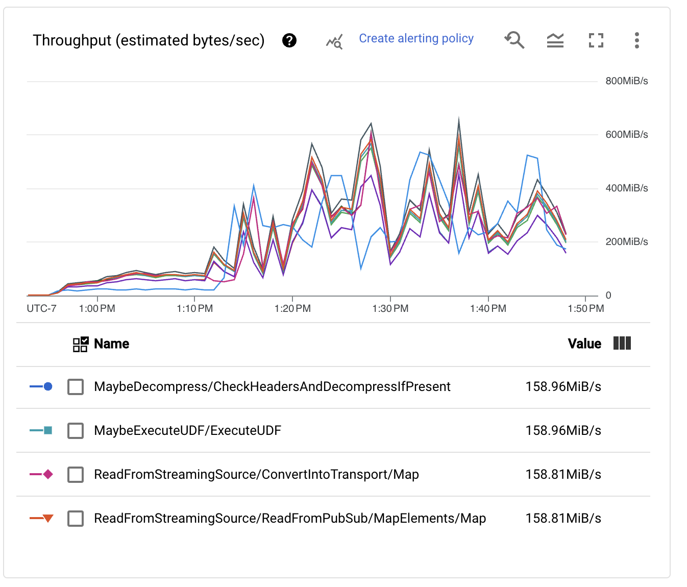
Although the performance has clearly improved, and the Pub/Sub backlog no longer increases monotonically, we are still far from the goal of processing one million events per second (1 GB/s) for our ingestion pipeline. In fact, the throughput metrics jump all over, indicating that bottlenecks are preventing the processing from scaling further.

Third run: unleash autoscale

Luckily for us, when writing into BigQuery, we can autoscale the writes. This step simplifies the configuration so that we don’t have to guess the right number of shards. We switched the pipeline’s configuration and enabled this setting for the next launch script.

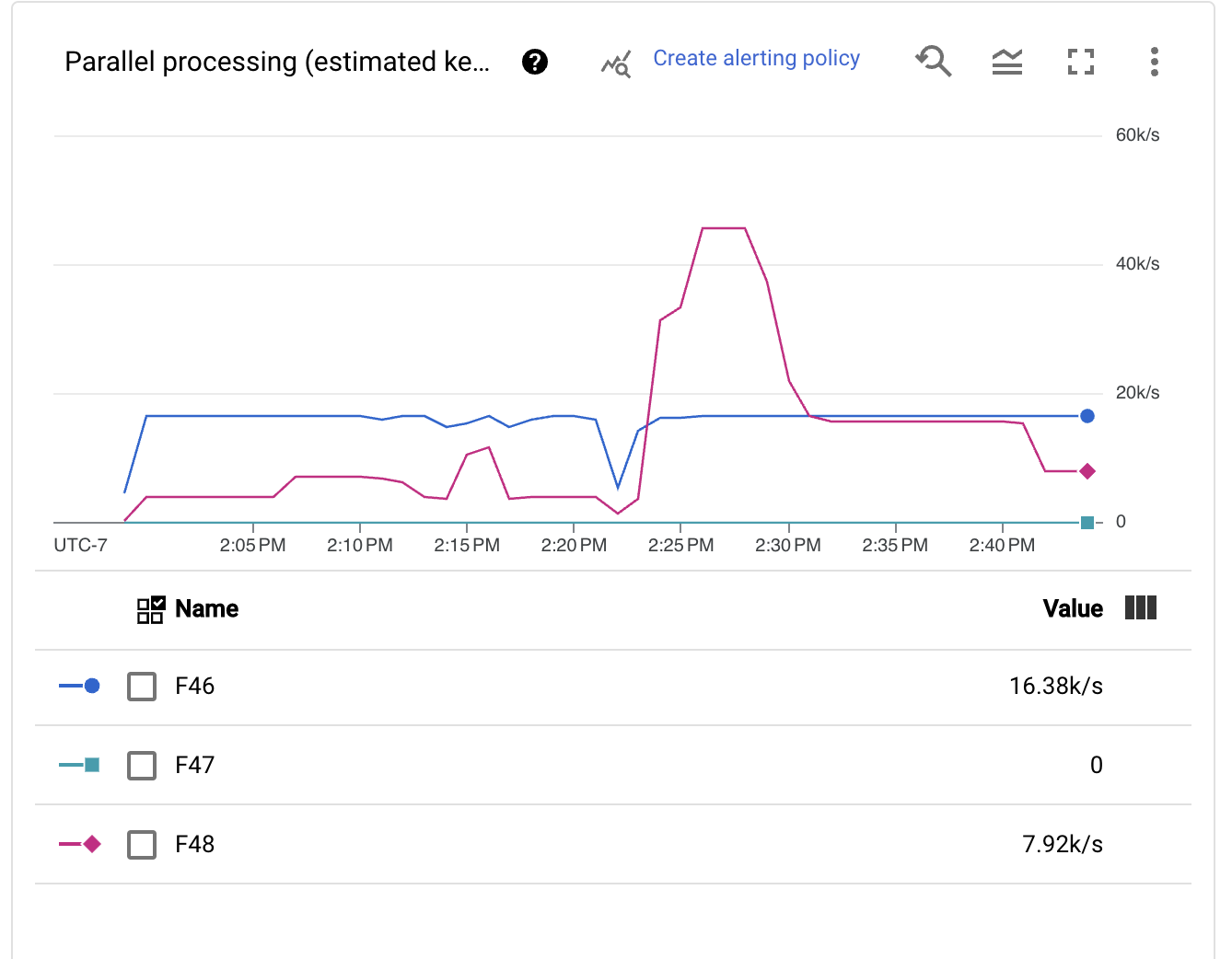
Immediately, we see that the autosharding mechanism tweaks the number of keys very aggressively and in a dynamic way. This change is good, because different moments in time might have different scale needs, such as early backlog recoveries and spikes in the execution.

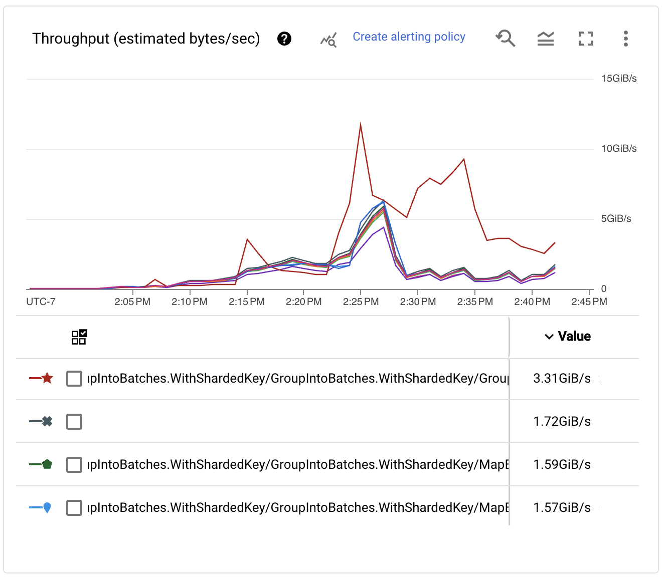
Inspecting the throughput performance per stage, we see that as the number of keys increases, the performance of the writes also increases. In fact, it reaches very large numbers!

After the initial backlog was consumed and the pipeline stabilized, we saw that the desired performance numbers were reached. The pipeline can sustain processing many more than a million events per second from Pub/Sub and several GB/s of BigQuery ingestion. Yay!

Still, we want to see if we can do better. We can introduce several improvements to the pipeline to make the execution more efficient. In most cases, the improvements are configuration changes. We just need to know where to focus next.

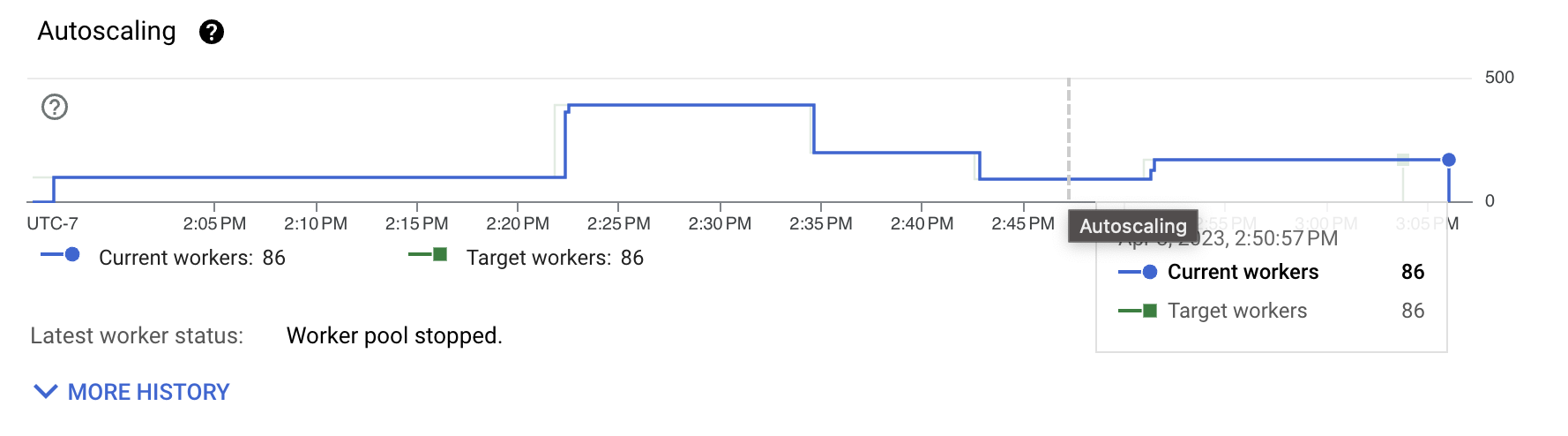
The previous image shows that the number of workers needed to sustain this throughput is still quite high. The workload itself is not CPU intensive. Most of the cost is spent on transforming formats and on I/O interactions, such as shuffles and the actual writes. To understand what to improve, we first investigate the transport formats.

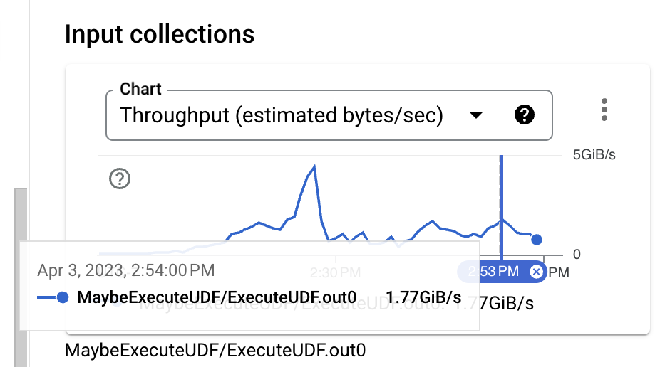
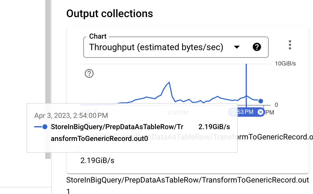
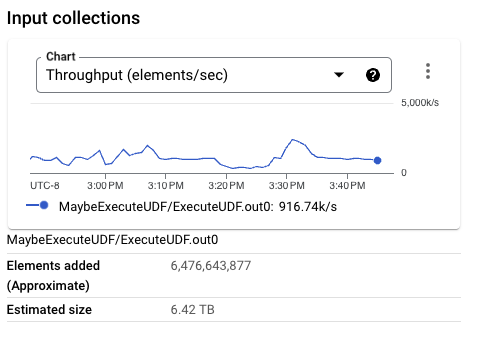
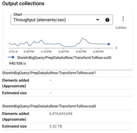
Looking at the input size, right before the identity UDF execution, the data format is binary Thrift, which is a decently compact format even when no compression is used. However, while comparing the PCollection approximated size with the TableRow format needed for BigQuery ingestion, a clear size increase is visible. This is something we can improve by changing the BigQuery write API in use.

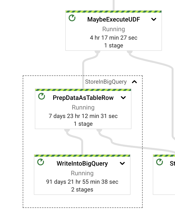
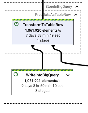
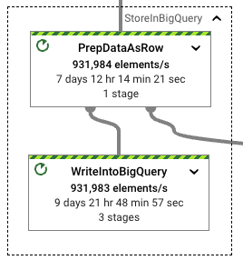
When we inspect the StoreInBigQuery transform, we see that the majority of the wall time is spent on the actual writes. Also, the wall time spent converting data to the destination format (TableRows) compared with how much is spent in the actual writes is quite large: 13 times bigger for the writes. To improve this behavior, we can switch the pipeline write mode.

Fourth run: in with the new

In this run, we use the StorageWrite API. Enabling the StorageWrite API for this pipeline is straightforward. We set the write mode as STORAGE_WRITE_API and define a write triggering frequency. For this test, we write data at most every ten seconds. The write triggering frequency controls how long the per-stream data accumulate. A higher number defines a larger output to be written after the stream assignment but also imposes a larger end-to-end latency for every element read from Pub/Sub. Similar to the STREAMING_WRITES configuration, BigQueryIO can handle autosharding for the writes, which we already demonstrated to be the best setting for performance.

After both pipelines become stable, the performance benefits seen when using the StorageWrite API in BigQueryIO are apparent. After enabling the new implementation, the wall time rate between the format transformation and write operation decreases. The wall time spent on writes is only about 34 percent larger than the format transformation.

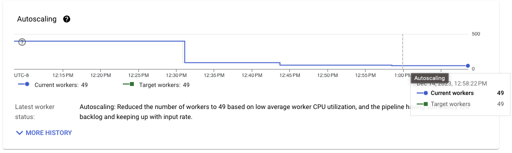
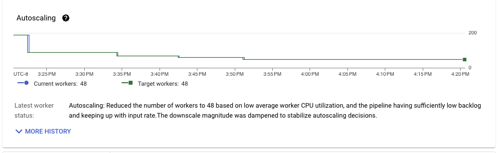
After stabilization, the pipeline throughput is also quite smooth. The runner can quickly and steadily downscale the pipeline resources needed to sustain the desired throughput.

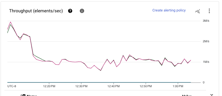
Looking at the resource scale needed to process the data, another dramatic improvement is visible. Whereas the streaming inserts-based pipeline needed more than 80 workers to sustain the throughput, the storage writes pipeline only needs 49, a 40 percent improvement.

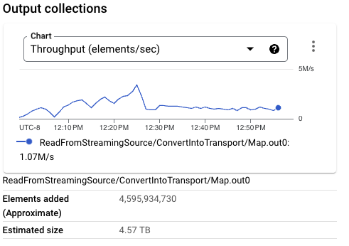
We can use the data generation pipeline as reference. This pipeline only needs to randomly generate data and write the events to Pub/Sub. It runs steadily with an average of 40 workers. The improvements on the ingestion pipeline using the right configuration for the workload makes it closer to those resources needed for the generation.

Similar to the streaming inserts-based pipeline, writing the data into BigQuery requires running a format translation, from Thrift to TableRow in the former and from Thrift to Protocol Buffers (protobuf) in the latter. Because we are using the BigQueryIO.writeTableRows method, we add another step in the format translation. Because the TableRow format also increases the size of the PCollection being processed, we want to see if we can improve this step.

Fifth run: a better write format

When using STORAGE_WRITE_API, the BigQueryIO transform exposes a method that we can use to write the Beam row type directly into BigQuery. This step is useful because of the flexibility that the row type provides for interoperability and schema management. Also, it’s both efficient for shuffling and denser than TableRow, so our pipeline will have smaller PCollection sizes.

For the next run, because our data volume is not small, we decrease the triggering frequency when writing to BigQuery. Because we use a different format, slightly different code runs. For this change, the test pipeline script is configured with the flag --formatToStore=BEAM_ROW.

The PCollection size written into BigQuery is considerably smaller than on previous executions. In fact, for this particular execution, the Beam row format is a smaller size than the Thrift format. A larger PCollection conformed by bigger per-element sizes can put nontrivial memory pressure in smaller worker configurations, reducing the overall throughput.

The wall clock rate for the format transformation and the actual BigQuery writes also maintain a very similar rate. Handling the Beam row format does not impose a performance penalty in the format translation and subsequent writes. This is confirmed by the number of workers in use by the pipeline when throughput becomes stable, slightly smaller than the previous run but clearly in the same range.

Although we are in a much better position than when we started, given our test pipeline input format, there’s still room for improvement.

Sixth run: further reduce the format translation effort

Another supported format for the input PCollection in the BigQueryIO transform might be advantageous for our input format. The method writeGenericRecords enables the transform to transform Avro GenericRecords directly into protobuf before the write operation. Apache Thrift can be transformed into Avro GenericRecords very efficiently. We can make another test run configuring our test ingestion pipeline by setting the option --formatToStore=AVRO_GENERIC_RECORD on our execution script.

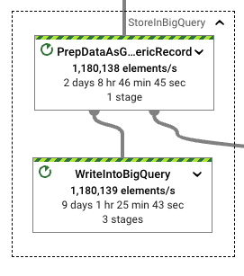
This time, the difference between format translation and writes increases significantly, improving performance. The translation to Avro GenericRecords is only 20 percent of the write effort spent on writing those records into BigQuery. Given that the test pipelines had similar runtimes and that the wall clock seen in the WriteIntoBigQuery stage is also aligned with other StorageWrite related runs, using this format is appropriate for this workload.

We see further gains when we look at resource utilization. We need less CPU time to execute the format translations for our workload while achieving the desired throughput.

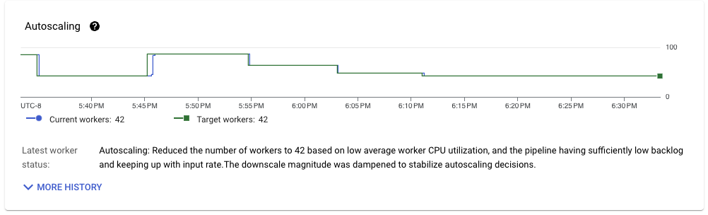
This pipeline improves upon the previous run, running steadily on 42 workers when throughput is stable. Given the worker configuration used (nd2-standard-4), and the volume throughput of the workload process (about 1 GB/s), we are achieving about 6 MB/s throughput per CPU core, which is quite impressive for a streaming pipeline with exactly-once semantics.

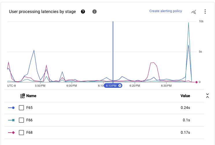
When we add up all of the stages executed in the main path of the pipeline, the latency seen at this scale achieves sub-second end-to-end latencies during sustained periods of time.

Given the workload requirements and the implemented pipeline code, this performance is the best that we can extract without further tuning the runner’s specific settings.

Seventh run : lets just relax (at least some constraints)

When using the STORAGE\_WRITE\_API setting for BigQueryIO, we enforce exactly-once semantics on the writes. This configuration is great for use cases that need strong consistency on the data that gets processed, but it imposes a performance and cost penalty.

From a high-level perspective, writes into BigQuery are made in batches, which are released based on the current sharding and the triggering frequency. If a write fails during the execution of a particular bundle, it is retried. A bundle of data is committed into BigQuery only when all the data in that particular bundle is correctly appended to a stream. This implementation needs to shuffle the full volume of data to create the batches that are written, and also the information of the finished batches for later commit (although this last piece is very small compared with the first).

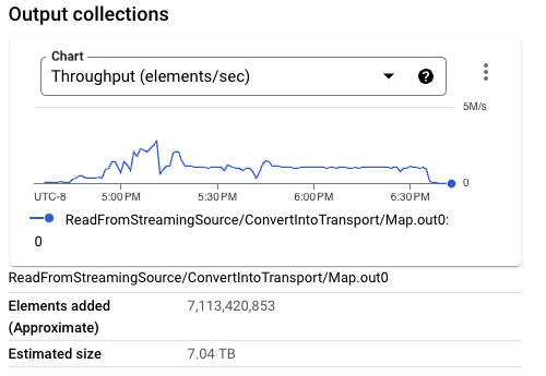
Looking at the previous pipeline execution, the total data being processed for the pipeline by Streaming Engine is larger than the data being read from Pub/Sub. For example, 7 TB of data is read from Pub/Sub, whereas the processing of data for the whole execution of the pipeline moves 25 TB of data to and from Streaming Engine.

When data consistency is not a hard requirement for ingestion, you can use at-least-once semantics with BigQueryIO write mode. This implementation avoids shuffling and grouping data for the writes. However, this change might cause a small number of repeated rows to be written into the destination table. This can happen with append errors, infrequent worker restarts, and other even less frequent errors.

Therefore, we add the configuration to use STORAGE_API_AT_LEAST_ONCE write mode. To instruct the StorageWrite client to reuse connections while writing data, we also add the configuration flag –useStorageApiConnectionPool. This configuration option only works with STORAGE_API_AT_LEAST_ONCE mode, and it reduces the occurrences of warnings similars to Storage Api write delay more than 8 seconds.

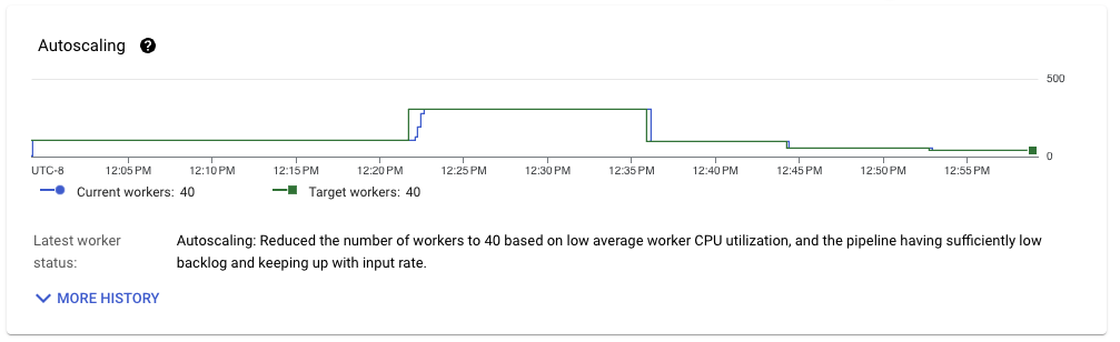
When pipeline throughput stabilizes, we see a similar pattern for resource utilization for the workload. The number of workers in use reaches 40, a small improvement compared with the last run. However, the amount of data being moved from Streaming Engine is much closer to the amount of data read from Pub/Sub.

Considering all of these factors, this change further optimizes the workload, achieving a throughput of 6.4 MB/s per CPU core. This improvement is small compared to the same workload when using consistent writes into BigQuery, but it uses less streaming data resources. This configuration represents the most optimal setup for our workload, with the highest throughput per resource and the lowest streaming data across workers.

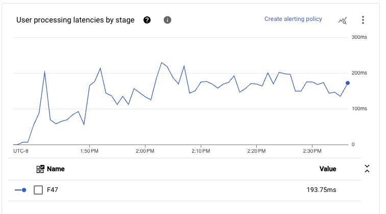
This configuration also has impressively low latency for the end-to-end processing. Given that the main path of our pipeline has been fused in a single execution stage from reads to writes, we see that even at p99, the latency tends to be below 300 milliseconds at a quite large volume throughput (as previously mentioned around 1 GB/s).

Recap

Optimizing Apache Beam streaming workloads for low latency and efficient execution requires careful analysis and decision-making, and the right configurations.

Considering the scenario discussed in this article, it is essential to consider factors like overall CPU utilization, throughput and latency per stage, PCollection sizes, wall time per stage, write mode, and transport formats, in addition to writing the right pipeline for the workload.

Our experiments revealed that using the StorageWrite API, autosharding for writes, and Avro GenericRecords as the transport format yielded the most efficient results. Relaxing the consistency for writes can further improve performance.

The accompanying Github repository contains a test suite that you can use to replicate the analysis on your Google Cloud project or with a different runner setup. Feel free to take it for a spin. Comments and PRs are always welcome.